import pandas as pd
import statsmodels.formula.api as smf
import numpy as np
import matplotlib.pyplot as plt

Panel data is a hybrid data type that has feature of both cross section and time series. Actually panel data are the most common data type in industry, for instance a car manufacturer has record of its suppliers’ price level over time, a bank has full history of its clients’ monthly balance for many years. Needless to say, to carry out serious researches, you must use panel data.

Here we will use the data from “Why has Productivity Declined? Productivity and Public Investment” written by Munell, A.

Variable names defined as below:

STATE = state name
ST_ABB = state abbreviation
YR = 1970,...,1986
P_CAP = public capital
HWY = highway capital
WATER = water utility capital
UTIL = utility capital
PC = private capital
GSP = gross state product
EMP = employment
UNEMP = unemployment rate

df = pd.read_excel(
    "../dataset/econometrics_practice_data.xlsx", sheet_name="Prod_PubInvestment"
)
df.head(5)

	STATE	YR	P_CAP	HWY	WATER	UTIL	PC	GSP	EMP	UNEMP
0	ALABAMA	1970	15032.67	7325.80	1655.68	6051.20	35793.80	28418	1010.5	4.7
1	ALABAMA	1971	15501.94	7525.94	1721.02	6254.98	37299.91	29375	1021.9	5.2
2	ALABAMA	1972	15972.41	7765.42	1764.75	6442.23	38670.30	31303	1072.3	4.7
3	ALABAMA	1973	16406.26	7907.66	1742.41	6756.19	40084.01	33430	1135.5	3.9
4	ALABAMA	1974	16762.67	8025.52	1734.85	7002.29	42057.31	33749	1169.8	5.5

df.tail(5)

	STATE	YR	P_CAP	HWY	WATER	UTIL	PC	GSP	EMP	UNEMP
811	WYOMING	1982	4731.98	3060.64	408.43	1262.90	27724.96	13056	217.7	5.8
812	WYOMING	1983	4950.82	3119.98	445.59	1385.25	28586.46	11922	202.5	8.4
813	WYOMING	1984	5184.73	3195.68	476.57	1512.48	28794.80	12073	204.3	6.3
814	WYOMING	1985	5448.38	3295.92	523.01	1629.45	29326.94	12022	206.9	7.1
815	WYOMING	1986	5700.41	3400.96	565.58	1733.88	27110.51	10870	196.3	9

Each state is recorded over time in several aspects, such as public capitals, highway capital, water facility capital and etc. If each state is recorded in equal length of time period, we call it balanced panel, otherwise unbalanced panel.

Estimation methods includes four approaches 1. Pooled OLS model 2. Fixed effects least square dummy variable (LSDV) model 3. Fixed effects within-in group model 4. Random effects model

Pooled OLS Regression

\[\begin{aligned} ln{GSP}_{i t} &=\beta_{1}+\beta_{2} \ln{PCAP}_{i t}+\beta_{3} \ln{HWY}_{i t}+\beta_{4} \ln{WATER}_{i t}+\beta_{5} \ln{UTIL}_{i t}+\beta_{6} \ln{EMP}_{i t}+u_{i t} \end{aligned}\]

where \(i\) means the \(i\)the state, \(t\) means time period.

model = smf.ols(
    formula="np.log(GSP) ~ np.log(P_CAP) + np.log(PC) + np.log(HWY) + np.log(WATER) + np.log(UTIL) + np.log(EMP)",
    data=df,
)
results = model.fit()
print(results.summary())

                            OLS Regression Results                            
==============================================================================
Dep. Variable:            np.log(GSP)   R-squared:                       0.993
Model:                            OLS   Adj. R-squared:                  0.993
Method:                 Least Squares   F-statistic:                 1.971e+04
Date:                Sun, 27 Oct 2024   Prob (F-statistic):               0.00
Time:                        17:36:44   Log-Likelihood:                 862.28
No. Observations:                 816   AIC:                            -1711.
Df Residuals:                     809   BIC:                            -1678.
Df Model:                           6                                         
Covariance Type:            nonrobust                                         
=================================================================================
                    coef    std err          t      P>|t|      [0.025      0.975]
---------------------------------------------------------------------------------
Intercept         1.2474      0.111     11.245      0.000       1.030       1.465
np.log(P_CAP)     0.7432      0.109      6.824      0.000       0.529       0.957
np.log(PC)        0.3124      0.011     28.553      0.000       0.291       0.334
np.log(HWY)      -0.3289      0.060     -5.520      0.000      -0.446      -0.212
np.log(WATER)     0.0276      0.018      1.568      0.117      -0.007       0.062
np.log(UTIL)     -0.3036      0.047     -6.510      0.000      -0.395      -0.212
np.log(EMP)       0.5932      0.016     36.761      0.000       0.561       0.625
==============================================================================
Omnibus:                       17.950   Durbin-Watson:                   0.200
Prob(Omnibus):                  0.000   Jarque-Bera (JB):               19.040
Skew:                           0.328   Prob(JB):                     7.34e-05
Kurtosis:                       3.360   Cond. No.                     1.23e+03
==============================================================================

Notes:
[1] Standard Errors assume that the covariance matrix of the errors is correctly specified.
[2] The condition number is large, 1.23e+03. This might indicate that there are
strong multicollinearity or other numerical problems.

The common symptoms of pooled regression on panel data is that all most of coefficients will be highly significant and also \(R^2\) is exceedingly high. However, we can still spot some problems, the conditional number is high, meaning multicollinearity and Durbin-Watson test is close to \(0\) meaning autocorrelation or specification error.

But the most prominent issue of this model is that it camouflages the heterogeneity that may exist among states. The heterogeneity of each state is subsumed by the disturbance term, which causes correlation between independent variables and disturbance terms, therefore OLS estimates are bound to be biased and inconsistent.

The Fixed Effect LSDV Model

LSDV model allows heterogeneity to take part in by adding different intercept value

\[\begin{aligned} ln{GSP}_{i t} &=\beta_{1i}+\beta_{2} \ln{PCAP}_{i t}+\beta_{3} \ln{HWY}_{i t}+\beta_{4} \ln{WATER}_{i t}+\beta_{5} \ln{UTIL}_{i t}+\beta_{6} \ln{EMP}_{i t}+u_{i t} \end{aligned}\]

\(\beta_{1i}\) represents the intercept for each state \(i\). There are various possible reasons contributing to heterogeneity among states, such as population, average education level and urbanization rate, etc.

Fixed effect means that though each state has its own intercept, but it is time-invariant, i.e. constant over the time. If we assume time-variant intercept, the notation would be \(\beta_{1it}\)

df

	STATE	YR	P_CAP	HWY	WATER	UTIL	PC	GSP	EMP	UNEMP
0	ALABAMA	1970	15032.67	7325.80	1655.68	6051.20	35793.80	28418	1010.5	4.7
1	ALABAMA	1971	15501.94	7525.94	1721.02	6254.98	37299.91	29375	1021.9	5.2
2	ALABAMA	1972	15972.41	7765.42	1764.75	6442.23	38670.30	31303	1072.3	4.7
3	ALABAMA	1973	16406.26	7907.66	1742.41	6756.19	40084.01	33430	1135.5	3.9
4	ALABAMA	1974	16762.67	8025.52	1734.85	7002.29	42057.31	33749	1169.8	5.5
...	...	...	...	...	...	...	...	...	...	...
811	WYOMING	1982	4731.98	3060.64	408.43	1262.90	27724.96	13056	217.7	5.8
812	WYOMING	1983	4950.82	3119.98	445.59	1385.25	28586.46	11922	202.5	8.4
813	WYOMING	1984	5184.73	3195.68	476.57	1512.48	28794.80	12073	204.3	6.3
814	WYOMING	1985	5448.38	3295.92	523.01	1629.45	29326.94	12022	206.9	7.1
815	WYOMING	1986	5700.41	3400.96	565.58	1733.88	27110.51	10870	196.3	9

816 rows × 10 columns

fig, ax = plt.subplots(nrows=2, ncols=3, figsize=(18, 12))
ax[0, 0].scatter(df["GSP"], df["P_CAP"], c="r", s=5)
ax[0, 0].grid()
ax[0, 0].set_xlabel("Public Capital")
ax[0, 0].set_ylabel("Gross Regional Produce")

ax[0, 1].scatter(df["GSP"], df["HWY"], c="r", s=5)
ax[0, 1].grid()
ax[0, 1].set_xlabel("High Way Capital")
ax[0, 1].set_ylabel("Gross Regional Produce")

ax[0, 2].scatter(df["GSP"], df["WATER"], c="r", s=5)
ax[0, 2].grid()
ax[0, 2].set_xlabel("Water Facility")
ax[0, 2].set_ylabel("Gross Regional Produce")

ax[1, 0].scatter(df["GSP"], df["UTIL"], c="r", s=5)
ax[1, 0].grid()
ax[1, 0].set_xlabel("Utiltiy Capital")
ax[1, 0].set_ylabel("Gross Regional Produce")

ax[1, 1].scatter(df["GSP"], df["PC"], c="r", s=5)
ax[1, 1].grid()
ax[1, 1].set_xlabel("Private Capital")
ax[1, 1].set_ylabel("Gross Regional Produce")

ax[1, 2].scatter(df["GSP"], df["EMP"], c="r", s=5)
ax[1, 2].grid()
ax[1, 2].set_xlabel("Employement")
ax[1, 2].set_ylabel("Gross Regional Produce")

plt.show()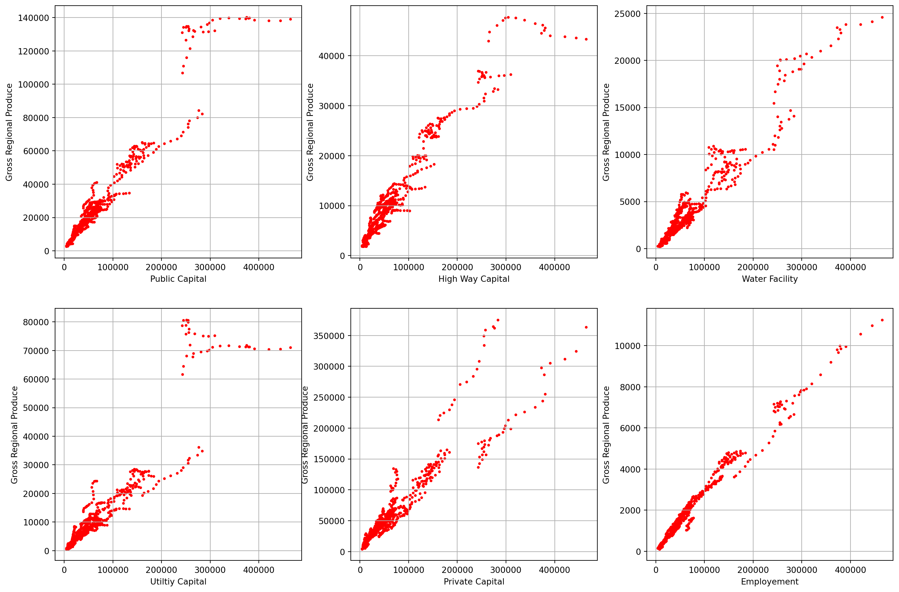

Check how many states are there in the panel data

print(df["STATE"].unique())
print(len(df["STATE"].unique()))

['ALABAMA' 'ARIZONA' 'ARKANSAS' 'CALIFORNIA' 'COLORADO' 'CONNECTICUT'
 'DELAWARE' 'FLORIDA' 'GEORGIA' 'IDAHO' 'ILLINOIS' 'INDIANA' 'IOWA'
 'KANSAS' 'KENTUCKY' 'LOUISIANA' 'MAINE' 'MARYLAND' 'MASSACHUSETTS'
 'MICHIGAN' 'MINNESOTA' 'MISSISSIPPI' 'MISSOURI' 'MONTANA' 'NEBRASKA'
 'NEVADA' 'NEW_HAMPSHIRE' 'NEW_JERSEY' 'NEW_MEXICO' 'NEW_YORK'
 'NORTH_CAROLINA' 'NORTH_DAKOTA' 'OHIO' 'OKLAHOMA' 'OREGON' 'PENNSYLVANIA'
 'RHODE_ISLAND' 'SOUTH_CAROLINA' 'SOUTH_DAKOTA' 'TENNESSE' 'TEXAS' 'UTAH'
 'VERMONT' 'VIRGINIA' 'WASHINGTON' 'WEST_VIRGINIA' 'WISCONSIN' 'WYOMING']
48

To avoid dummy variable trap, we can define \(47\) dummy intercepts.

Add dummies onto the intercept

\[\begin{aligned} ln{GSP}_{i t} &=\alpha_{1}+ \sum_{j=2}^{48}\alpha_{j} D_{j i}+\beta_{2} \ln{PCAP}_{i t}+\beta_{3} \ln{HWY}_{i t}+\beta_{4} \ln{WATER}_{i t}+\beta_{5} \ln{UTIL}_{i t}+\beta_{6} \ln{EMP}_{i t}+u_{i t} \end{aligned}\]

Use STATE as the dummy column and add drop_fist to avoid dummy trap.

df_dum = pd.get_dummies(data=df, columns=["STATE"], drop_first=True)

df_dum

	YR	P_CAP	HWY	WATER	UTIL	PC	GSP	EMP	UNEMP	STATE_ARIZONA	...	STATE_SOUTH_DAKOTA	STATE_TENNESSE	STATE_TEXAS	STATE_UTAH	STATE_VERMONT	STATE_VIRGINIA	STATE_WASHINGTON	STATE_WEST_VIRGINIA	STATE_WISCONSIN	STATE_WYOMING
0	1970	15032.67	7325.80	1655.68	6051.20	35793.80	28418	1010.5	4.7	False	...	False	False	False	False	False	False	False	False	False	False
1	1971	15501.94	7525.94	1721.02	6254.98	37299.91	29375	1021.9	5.2	False	...	False	False	False	False	False	False	False	False	False	False
2	1972	15972.41	7765.42	1764.75	6442.23	38670.30	31303	1072.3	4.7	False	...	False	False	False	False	False	False	False	False	False	False
3	1973	16406.26	7907.66	1742.41	6756.19	40084.01	33430	1135.5	3.9	False	...	False	False	False	False	False	False	False	False	False	False
4	1974	16762.67	8025.52	1734.85	7002.29	42057.31	33749	1169.8	5.5	False	...	False	False	False	False	False	False	False	False	False	False
...	...	...	...	...	...	...	...	...	...	...	...	...	...	...	...	...	...	...	...	...	...
811	1982	4731.98	3060.64	408.43	1262.90	27724.96	13056	217.7	5.8	False	...	False	False	False	False	False	False	False	False	False	True
812	1983	4950.82	3119.98	445.59	1385.25	28586.46	11922	202.5	8.4	False	...	False	False	False	False	False	False	False	False	False	True
813	1984	5184.73	3195.68	476.57	1512.48	28794.80	12073	204.3	6.3	False	...	False	False	False	False	False	False	False	False	False	True
814	1985	5448.38	3295.92	523.01	1629.45	29326.94	12022	206.9	7.1	False	...	False	False	False	False	False	False	False	False	False	True
815	1986	5700.41	3400.96	565.58	1733.88	27110.51	10870	196.3	9	False	...	False	False	False	False	False	False	False	False	False	True

816 rows × 56 columns